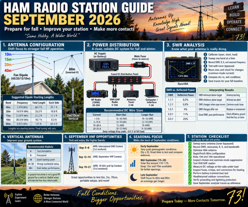
Monthly focus:shift the station toward stronger fall HF operation, prepare 40 and 80 meters for longer evenings, verify DC-power reliability before colder weather, and establish a clean SWR baseline after summer heat and thunderstorms.
September 2026 opens with unusually quiet space-weather conditions. NOAA’sSeptember 1, 2026three-day forecast expects Kp to remain at or below 2 through September 3, with no G1-or-greater geomagnetic storms expected and only a 10% daily chance of R1–R2 radio blackouts. NOAA’s September 1 longer-range forecast places the F10.7 solar flux mostly around95–115 through much of September, with the stronger portion currently forecast around September 15–20.
That makes September a particularly useful month for comparing antennas under relatively stable conditions rather than assuming every signal change is caused by propagation.
1. September Antenna Configuration
The seasonal priority should begin moving away from a summer emphasis on 6 and 10 meters and toward20, 40, and eventually 80 meters, while keeping the higher bands available whenever conditions support them.
Band
September role
Recommended configuration
80m
Evening/night regional work
Dipole, inverted-V, loaded dipole
40m
Major evening/night band
Dipole, fan dipole, EFHW, vertical
20m
Daytime and early-evening DX
Dipole, vertical, beam
15m
Opportunistic daytime DX
Fan-dipole element or dedicated antenna
10m
Check during stronger solar periods
Dipole, vertical, small beam
6m
Less seasonal Es, but still useful
Horizontal dipole, Moxon, Yagi
2m/70cm
Repeaters, local work, VHF contest
Vertical plus horizontal antenna if possible
For a general-purpose September station, a very effective combination is a40/20/15/10-meter fan dipole plus a separate 80-meter antenna. Trying to place every HF band on one compact fan structure often creates more interaction than it solves.
2. Prepare 40 Meters First
September is an excellent month to optimize 40 meters because darkness is arriving earlier and the band becomes increasingly useful during evening operating.
For a dipole centered near the FT8 frequency of7.074 MHz, the standard 468/f starting formula gives approximately:
66.2 feet total, or about33.1 feet per side.
For a more general SSB-oriented antenna centered near 7.200 MHz, the starting length is approximately65 feet total.
These are construction starting points, not final dimensions. Wire insulation, height, nearby buildings, trees, gutters, attic materials, and element interaction can all shift resonance.
For an inverted-V, keep the feedpoint as high as practical and avoid extremely acute angles between the legs. The ends can be lower, but keep them away from people and conductive objects.
3. Begin 80-Meter Preparation
If you want improved fall and winter regional coverage, September is the month to begin 80-meter work rather than waiting until November.
At approximately3.573 MHz, an FT8-centered half-wave dipole starts near131 feet total. Many residential properties cannot accommodate that straight-line span, so practical alternatives include an inverted-V, bent dipole, loaded dipole, shortened antenna, or a carefully designed multiband system.
Do not judge an 80-meter antenna solely by SWR. A heavily shortened antenna can present an attractive 1.2:1 match while still suffering substantial loading-coil or ground loss.
For lower HF bands,efficiency and radiation resistance matter more than obtaining a perfect meter reading.
4. Keep 15 and 10 Meters Available
NOAA’s September 1 forecast has solar flux increasing from approximately 95–105 during the first half of September toward110–115 around September 15–20, before easing toward the end of the month.
Do not dismantle your higher-band antennas yet.
During the stronger part of the forecast period, check:
Band
Digital calling area to monitor
20m FT8
14.074 MHz
15m FT8
21.074 MHz
10m FT8
28.074 MHz
6m FT8
50.313 MHz
Even when a band sounds silent on SSB, digital monitoring can reveal propagation that is not obvious by listening.
5. September Fan-Dipole Configuration
A useful three-band or four-band fan dipole can begin with these approximate dimensions:
Band
Frequency
Total starting length
Each side
40m
7.074 MHz
66.2 ft
33.1 ft
20m
14.074 MHz
33.3 ft
16.6 ft
15m
21.074 MHz
22.2 ft
11.1 ft
10m
28.074 MHz
16.7 ft
8.3 ft
Leave the wires slightly long.
Tune from thelowest-frequency element upward:
40m → 20m → 15m → 10m
After adjusting each higher-frequency element, sweep the lower bands again. Fan-dipole elements are electromagnetically coupled, so changing one wire can shift another.
Place a1:1 current chokenear the feedpoint. ARRL notes that dipoles and other complete antennas generally do not require an RF ground when common-mode feed-line currents are properly controlled; current or choke baluns are commonly used for this purpose. (ARRL)
6. September Vertical-Antenna Work
Late summer is a good opportunity to inspect a vertical before leaves, wet ground, frost, and winter weather complicate maintenance.
Do not use SWR as the sole measure of vertical performance. A lossy ground system can produce deceptively good SWR because ground resistance becomes part of the feedpoint resistance.
For a ground-mounted quarter-wave vertical, concentrate on repairing or expanding the radial field.
Ground system
Practical interpretation
4 radials
Test installation
8 radials
Functional
16 radials
Good practical starting point
24–32 radials
Strong residential installation
48+ radials
Increasingly serious ground system
ARRL specifically notes that a ground rod by itself provides relatively high RF resistance for a quarter-wave vertical and that radial wires provide the lower-loss return path the antenna needs. (ARRL)
7. September VHF Opportunity
September is not exclusively an HF month.
The2026 ARRL September VHF Contest runs from 1800 UTC September 12 through 0259 UTC September 14and uses authorized amateur frequencies above 50 MHz. It is an excellent reason to test 6 meters, 2 meters, 70 centimeters, grid-square logging, portable antennas, and horizontal polarization. (ARRL Contests)
ARRL also has its second International EME Contest weekend onSeptember 5–6and the second 10 GHz and Up weekend onSeptember 19–21. (ARRL Contests)
Even without EME or microwave equipment, increased contest activity makes September a useful time to evaluate VHF receive performance.
8. Power Distribution: September Reliability Check
September should be the month when the station’s DC system receives a complete inspection before winter.
A clean station topology is:
AC supply or battery → main protection → fused DC distribution → separately fused equipment branches
A star configuration is preferable to daisy-chaining equipment.
For a typical 100-watt HF station, use the radio manufacturer’s maximum-current specification when sizing conductors. Many 100-watt HF radios require approximately 20–25 amps at full output, so voltage drop can become significant even when the power supply itself is functioning correctly.
A useful planning guide is:
Load
Short DC run
Longer DC run
Under 5 A
16–18 AWG
14–16 AWG
5–10 A
14–16 AWG
12–14 AWG
15–20 A
12 AWG
10 AWG
20–25 A
10–12 AWG
8–10 AWG
These are station-planning examples rather than universal electrical requirements. Cable length, insulation rating, allowable voltage drop, connectors, and manufacturer requirements still matter.
9. Measure Voltage at the Radio
One of the most useful station diagnostics is often overlooked.
Measure voltage directly at the radio’s DC connector under these conditions:
Test
Record
Radio off
Supply voltage
Receive
Radio-terminal voltage
25W transmit
Voltage
50W transmit
Voltage
100W transmit
Voltage
Several FT8 cycles
Voltage and connector temperature
Suppose your power supply reads13.8 Vbut your transceiver receives only12.7 V during transmit. The supply may not be the problem.
A surprisingly small amount of resistance becomes important at 20 amps.
For example, only 0.05 ohm of unwanted resistance causes:
V = I × R = 20 × 0.05 = 1 volt
of voltage loss.
It also produces:
P = I²R = 20² × 0.05 = 20 watts
of heat at the unwanted resistance.
That is why a marginal crimp or fuse holder can become very hot even though the cable itself appears properly sized.
10. September Backup-Power Exercise
Before winter, perform one controlled battery test.
Do not merely confirm that the battery shows the correct resting voltage. Put the station under an actual transmitter load.
Record battery voltage at receive, 25 watts, 50 watts, and your normal operating power.
For portable or emergency setups, fuse the positive battery lead close to the source. A battery can deliver enormous fault current into a short circuit.
Also inspect polarity labels, Powerpole housings, crimp integrity, charger condition, cable abrasion, and battery terminals.
11. September SWR Baseline
September is particularly well suited to creating yourfall antenna reference measurements.
Take the tuner completely out of the initial test.
For each antenna, record:
Parameter
Why it matters
Lowest SWR
Basic matching reference
Frequency of minimum SWR
Shows resonance movement
SWR at operating frequency
Actual station condition
R
Resistive component
X
Reactive component
Band-edge SWR
Indicates usable bandwidth
Ambient condition
Helps identify environmental changes
Coax configuration
Necessary for repeatable comparison
Analyzer calibration point
Defines measurement plane
This baseline becomes extremely valuable in November or January when an antenna suddenly appears different.
12. Understanding SWR Correctly
SWR doesnotdirectly tell you antenna efficiency.
Approximate reflected-power values are:
SWR
Reflected power
1.1:1
0.2%
1.2:1
0.8%
1.5:1
4%
2.0:1
11%
3.0:1
25%
This is why a stable1.5:1antenna normally does not justify drastic changes merely to reach 1.0:1.
It is also why a suddenly changing 1.5:1 reading is more interesting than a stable 2.0:1 reading that has always characterized the antenna.
Trend matters.
13. Separate the Tuner from the Antenna
An antenna tuner can make the transceiver see a low SWR without changing the SWR on the transmission line between the tuner and antenna.
ARRL gives the example of a2.5:1 antenna/feed-line SWR: after the tuner produces approximately 1:1 at the transmitter, the line between the tuner and antenna still operates at 2.5:1. Additional feed-line loss can result, particularly at higher frequencies and with lossy coax. (ARRL)
For diagnostics, always sweep the antenna with the tuner bypassed first.
14. NanoVNA / Analyzer Workflow
For repeatable September measurements, use the same procedure every time.
Calibrate usingopen, short, and 50-ohm load at the measurement plane. If you are using a jumper cable between the analyzer and antenna, calibrate at the far end of that jumper.
Then sweep only the band under test rather than 1–30 MHz all at once.
For example, examine 40 meters over approximately:
6.8–7.5 MHz
instead of trying to interpret a tiny 40-meter feature on a 30 MHz-wide screen.
Record the frequency where reactance approaches zero as well as the frequency where SWR reaches minimum. They are often close but are not necessarily identical.
15. Diagnose Resonance Movement
Use this simple interpretation:
Measurement
Likely condition
SWR minimum below desired frequency
Antenna electrically too long
SWR minimum above desired frequency
Antenna electrically too short
SWR changes when coax moves
Common-mode current or connection issue
SWR changes after rain
Moisture or environmental coupling
SWR rises during extended transmit
Heating component
SWR suddenly becomes very high
Connector, feed line, matching network, or antenna fault
SWR remains good but received signals fall
Do not assume antenna is healthy
When trimming a dipole, remove equal amounts from both ends and make increasingly small adjustments as you approach the desired frequency.
16. Check for Common-Mode Current
A particularly useful September test is to sweep the antenna, then gently reroute the coax.
If resonance or SWR changes appreciably merely because the feed line moved, the coax may be functioning as part of the antenna.
Other warning signs include computer USB problems during transmission, RF on microphone housings, distorted transmit audio, tuner settings changing when cables are moved, or interference with nearby electronics.
The preferred fix is generally to correct the antenna’s feed and install an appropriatecommon-mode choke, rather than attempting to solve the problem with an arbitrary shack-ground wire.
17. Post-Summer Feed-Line Inspection
Summer storms, ultraviolet exposure, wind, and water can expose weak connectors.
Before fall, inspect every accessible outdoor connection.
Pay particular attention to a connector whose SWR changes after rainfall and slowly returns to normal after several dry days. That pattern is strongly suggestive of moisture involvement.
A dummy-load substitution test can help isolate the problem.
Disconnect the antenna at the far end of the feed line and install a known-good 50-ohm load. Then measure from the shack.
If the system now shows a very low SWR, concentrate on the antenna or matching system.
If it still shows abnormal SWR, concentrate on coax, connectors, adapters, or the measurement setup.
18. Grounding and Lightning Protection
Thunderstorm risk does not disappear simply because August is over.
ARRL distinguisheselectrical-safety grounding, lightning protection, and RF-current managementas separate functions. One grounding arrangement should not be assumed to solve all three. (ARRL)
September is a good time to inspect bonding, coax surge protectors, ground conductors, weatherproofing, cable-entry hardware, and antenna supports before cold weather.
Avoid adding an isolated ground rod as an RF experiment without understanding how it must be bonded to the building grounding electrode system. Electrical-code and lightning-protection work should follow applicable standards and qualified guidance.
September Operating Plan
September 1–7:Establish your HF baseline while NOAA currently expects very quiet geomagnetic conditions through September 3. Sweep 40, 20, 15, and 10 meters before making antenna changes.
September 8–14:Concentrate on VHF and antenna comparisons. The ARRL September VHF Contest runs September 12–14, providing increased activity above 50 MHz. (ARRL Contests)
September 15–21:Keep 15 and 10 meters available. NOAA’s September 1 forecast currently places the month’s stronger F10.7 values, approximately 110–115, in this period. Treat that as planning guidance rather than a guarantee.
September 22–30:Shift attention toward 40 and 80 meters. Complete feed-line weatherproofing, battery testing, grounding inspection, and your fall SWR baseline before temperatures fall.
September Priority Checklist
Sweep every antenna with the tuner bypassed.
Record minimum SWR, resonance, R, X, and bandwidth.
Optimize the 40-meter antenna.
Begin or finish the 80-meter fall configuration.
Keep 15m and 10m operational for favorable openings.
Inspect feedpoint chokes and common-mode suppression.
Test the VHF/UHF station before September 12.
Measure DC voltage at the radio under full transmit load.
Inspect fuse holders, crimps, Powerpole connections, and cables for heating.
Perform a real battery transmit-load test.
Inspect outdoor coax weatherproofing.
Verify station grounding and lightning-protection bonding.
Save September analyzer traces as the fall reference.
The central goal forSeptember 2026is not to chase the lowest possible SWR. It is to build arepeatable, measurable station baseline. If you know what the antenna impedance, feed-line behavior, transmitter voltage, and normal operating temperatures look like now, troubleshooting through fall and winter becomes dramatically easier.
Here is a learning idea for Schaumburg Amateur Radio Club (SARC), N9RJV: explore the history behind the mathematics we use to understand radio. You do not need advanced math to begin. Start with counting, follow the development of patterns and proof, and discover how ideas from many cultures connect to waves, calculations, and communication.
Topic Snapshot
Topic at a glance
Item
Details
Subject
The History of Mathematics: From Early Counting to Modern Research
Club
Schaumburg Amateur Radio Club, N9RJV
Post idea
Paul Meyers – KE9EJX
Audience
Members, visitors, new hams, the public, operators, and volunteers
Format
A historical overview with optional learning activities and discussion ideas
Starting point
Curiosity, basic arithmetic, and a willingness to ask questions
Radio connections
Measurement, frequency, wavelength, oscillations, information, and careful reasoning
Read this as a journey, or choose one section that catches your interest. BCE means “Before Common Era,” and CE means “Common Era.” These labels use the same year numbering as BC and AD.
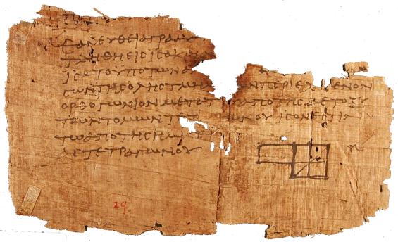
Above: a surviving papyrus fragment of Euclid’s Elements, found at Oxyrhynchus in Egypt. It illustrates an important feature of mathematical history: our knowledge depends partly on which documents happened to survive.[1]
Mathematics has no single inventor, birthplace, or straight-line history. It developed through many cultures, sometimes independently and sometimes through translation, trade, migration, teaching, and collaboration. Its history includes practical calculation, abstract reasoning, measurement, astronomy, games, commerce, and the study of patterns. [2]
The clearest way to understand this enormous subject is to follow two connected stories: how mathematical ideas developed over time, and how those ideas became the branches of mathematics we recognize today.
This account covers the main traditions, turning points, and families of mathematics. Dates for ancient developments are approximate, and the earliest surviving evidence is not necessarily the moment an idea was first conceived.
1. Before written mathematics: quantity, pattern, and measurement
Mathematics begins with ideas simpler than written numerals: distinguishing one object from several, comparing quantities, matching objects one-to-one, recognizing repeated patterns, and keeping track of sequences.
An important distinction is between having a concept of quantity and having a written number system. A community can count effectively through spoken words, fingers, arrangements of objects, or other memory aids without writing equations. Research on traditional counting systems demonstrates considerable mathematical sophistication outside written notation. [3]
Prehistoric artifacts sometimes contain repeated marks that may have served numerical purposes. The Ishango bone, found in Central Africa, is a famous example. However, interpretations of its marks—as tallying, arithmetic, calendrical recording, or something else—remain disputed. It should not be presented as conclusive evidence that prehistoric people understood prime numbers or possessed a particular advanced mathematical theory. [4]
The important transition was not simply “people started counting.” It was that quantities could be represented, remembered, compared, and manipulated independently of the objects themselves.
That is the beginning of abstraction: “five” becomes something shared by five stones, five animals, and five days.
2. Mesopotamia: written calculation and place value
Especially the third and second millennia BCE
Some of the earliest extensive written mathematical evidence comes from Mesopotamia, including Sumerian and Babylonian traditions.
Surviving clay tablets show arithmetic tables, calculations involving reciprocals and square roots, geometric problems, and procedures equivalent to solving certain linear and quadratic equations. Old Babylonian mathematics was already highly developed during approximately 2000–1600 BCE. [5]
A major innovation was place value: a symbol’s numerical contribution depended on its position.
Babylonian calculation used a base-60, or sexagesimal, system. Our divisions of angles into degrees, minutes, and seconds preserve part of that sexagesimal inheritance. This was not identical to modern decimal notation: conventions for empty positions and numerical scale developed over time. [5]
Babylonian tablets also demonstrate knowledge of numerical relationships between the sides of right triangles long before Pythagoras. For example, in modern notation:
32 + 42 = 52.
The modern equation is a translation of the relationship, not the notation Babylonian scribes used. Their mathematics often appeared as worked numerical procedures rather than symbolic formulas. [5]
What developed here: systematic arithmetic, computational algorithms, practical geometry, and procedures that later historians recognize as algebraic.
3. Egypt: fractions, surveying, and practical geometry
Especially the second millennium BCE
Egyptian mathematics is known largely through surviving papyri, particularly the Rhind Mathematical Papyrus, copied by the scribe Ahmes around 1650 BCE, and the Moscow Mathematical Papyrus, generally associated with an earlier period around 1850 BCE. The Rhind manuscript itself states that it draws on older material. [6]
The problems concern distributing food, calculating quantities of grain, measuring fields, and finding areas and volumes. They also include exercises designed to teach calculation itself.
Egyptian arithmetic made extensive use of unit fractions, fractions with a numerator of one, such as 1/2, 1/3, and 1/10. Multiplication could be performed through doubling and addition. These methods may look unfamiliar today, but they formed a workable computational system. [6]
An important lesson is that mathematical sophistication does not require modern notation. A procedure written in words can embody substantial reasoning.
What developed here: fraction arithmetic, proportional reasoning, measurement, and geometric calculation.
4. Greek and Hellenistic mathematics: the organization of proof
Approximately 600 BCE–500 CE
Greek-language mathematics introduced a particularly influential way of organizing knowledge: starting with definitions and assumptions, then developing a connected sequence of demonstrations.
Around 300 BCE, Euclid’s Elements assembled geometry, proportion, and number theory into an extensive deductive structure. Euclid did not invent everything in the work; much of his achievement lay in selection, organization, and logical presentation. [7]
The distinction between an example and a proof became especially important. Checking many triangles is not the same as demonstrating that a relationship holds for every triangle satisfying specified assumptions.
Greek mathematics also confronted incommensurable magnitudes: lengths that cannot be expressed as a ratio of whole numbers. The diagonal of a unit square, represented today by √2, is a familiar example. Euclid’s treatment of proportion and magnitudes provided ways to reason about such quantities without modern real-number notation. [7]
Archimedes, in the third century BCE, developed powerful methods for areas, volumes, centers of gravity, and approximations to π. His work combined mechanical insight with rigorous geometric argument. Methods that squeeze a quantity between increasingly close bounds anticipate important themes in later analysis, although they were not modern calculus. [8]
Astronomy also encouraged the development of trigonometric techniques, including Greek chord tables. These ideas would later be transformed by Indian and Islamic mathematicians. [9]
It would be misleading, however, to say that Greeks invented all mathematical reasoning or that other traditions merely calculated. Chinese mathematical commentaries, for example, also contain substantial demonstrations and explanations. [10]
5. China: algorithms, negative numbers, and systems of equations
Ancient foundations through the medieval period
Chinese mathematics developed a strong tradition of computational procedures, often using counting rods arranged on a surface.
A central text is The Nine Chapters on the Mathematical Art, compiled from material accumulated over time. Its problems include fractions, proportions, land measurement, roots, volumes, and simultaneous equations. Liu Hui’s commentary of 263 CE supplies explanations and geometric reasoning that help reveal why the procedures work. [10]
One especially important development was a systematic method for eliminating unknowns from several equations. In modern language, this is closely related to the elimination methods taught in linear algebra.
The text also includes rules involving positive and negative quantities. This is a reminder that the acceptance and use of negative numbers did not follow the same timetable everywhere. [10]
Later Chinese mathematicians developed sophisticated work on polynomial equations, numerical root-finding, and remainder problems. Scholars such as Qin Jiushao and Zhu Shijie contributed to a substantial medieval algebraic tradition. [11]
In Japan, the later wasan tradition developed its own distinctive mathematical culture. Seki Takakazu, in the seventeenth century, made important contributions to algebraic and computational methods. [12]
What developed here: algorithmic mathematics, numerical methods, signed arithmetic, equation systems, and polynomial techniques.
6. India: geometry, decimal numerals, zero, and infinite series
First millennium BCE–sixteenth century CE
Indian mathematics developed through several overlapping traditions, including ritual geometry, astronomy, arithmetic, algebra, and the analysis of patterns.
The Śulbasūtras, composed during the first millennium BCE, contain geometric construction rules associated with ritual altars. They address transformations between shapes, right-triangle relationships, and approximations needed for construction. [13]
Decimal place value and zero
Indian mathematical traditions were central to the development of the decimal place-value system that eventually became widely used internationally.
But “the invention of zero” is not one event. A mark for an empty position, the idea of an absent quantity, and zero treated as a number in arithmetic are related but distinct developments. The system evolved over centuries. [14]
In 628 CE, Brahmagupta stated influential arithmetic rules involving zero and positive and negative quantities. His rules were not identical to the complete modern system: division involving zero remained problematic. His work also included equations and number-theoretic problems. [15]
Trigonometry and astronomy
Indian astronomer-mathematicians, including Aryabhata, developed sine-based methods that differed from the Greek use of chords. These techniques became important in the subsequent development of trigonometry across the Islamic world and Europe. [9]
The Kerala school
Around the late fourteenth and early fifteenth centuries, Madhava of Sangamagrama developed results involving infinite series for trigonometric functions and π. Much of our knowledge of his mathematics comes through later members of the Kerala school.
The school’s work included sophisticated reasoning about approximation and correction terms. These were major achievements in the history of infinite processes. They should neither be overlooked nor automatically equated with the entire general framework of seventeenth-century calculus. [16]
7. The Islamic world: algebra, trigonometry, and mathematical synthesis
Approximately 750–1500 CE
Across a wide region—from Central Asia and Persia through the Middle East and North Africa to al-Andalus—scholars translated, studied, criticized, and extended Greek, Indian, and other mathematical works.
This was not merely a period of preservation. Original developments occurred in algebra, number theory, geometry, trigonometry, and numerical calculation. The scholarly communities involved were multilingual and included people of different religious backgrounds. [17]
In the early ninth century, al-Khwarizmi presented a systematic treatment of linear and quadratic equations. His work organized equation-solving into recognizable classes and explained procedures, including geometric justifications.
The word algebra derives from al-jabr, part of the title of his work. The word algorithm ultimately derives from a Latinized form of his name. His writings on arithmetic also helped transmit Indian computational methods. [18]
Later developments included polynomial arithmetic associated with al-Karaji, geometric solutions of cubic equations by Omar Khayyam, and increasingly sophisticated plane and spherical trigonometry.
These subjects served astronomy and other practical purposes, but they also became areas of investigation in their own right. [17]
What developed here: a more systematic algebra, advanced trigonometry, numerical techniques, and influential connections among earlier mathematical traditions.
8. The Americas, Africa, and Oceania: other mathematical traditions
A global history must include mathematical knowledge that did not enter the familiar sequence of European textbooks.
Maya mathematics
Maya mathematics included positional numerical notation and a symbol for zero, used prominently in calendrical and astronomical calculations.
The system was largely based on twenties, but calendar-related notation included a modified place involving 18×20=360. It therefore should not be described simply as an unmodified base-20 system in every context. [19]
Andean mathematics
In the Inca world, khipu, also spelled quipu, encoded numerical information through knotted cords. Numerical khipu used decimal organization and supported recordkeeping and administration.
They demonstrate that numerical information can be represented structurally and physically, rather than exclusively through marks on a flat writing surface. [20]
African geometric traditions
The sona sand-drawing tradition associated with Chokwe communities in Angola includes geometric construction procedures, symmetries, and continuous-line patterns.
Research by Paulus Gerdes analyzed mathematical structures in these practices. Care is necessary: a modern mathematical analysis of a traditional design is not automatically evidence that its historical makers expressed the same ideas in modern terminology. Nevertheless, the procedures themselves are genuine objects of mathematical and historical interest. [21]
Polynesian counting
Research on Mangarevan counting documents a system combining decimal organization with binary steps. This is not the same as modern computer notation, but it demonstrates an ingenious way to simplify mental calculation without written numerals. [3]
Together, these examples challenge the assumption that mathematics exists only where there are textbooks, universities, or algebraic symbols.
9. Medieval and Renaissance Europe: translation and symbolic calculation
Approximately 1100–1650
Medieval European mathematics developed partly through translations and exchanges involving Arabic and Greek sources.
Leonardo of Pisa, known as Fibonacci, learned mathematical methods in North Africa. His Liber Abaci of 1202 helped introduce and explain Hindu-Arabic arithmetic to a Latin-reading audience, including its commercial applications. He did not invent the numerals or the decimal system. [22]
During the sixteenth century, work by del Ferro, Tartaglia, Cardano, and Ferrari produced methods for solving cubic and quartic equations. These investigations also forced mathematicians to confront expressions involving square roots of negative quantities. Bombelli helped develop systematic rules for handling them. [23]
Symbolic notation gradually became more compact and flexible. Letters increasingly represented unknowns and general quantities. The equals sign appeared in Robert Recorde’s work in 1557, while later authors helped establish other familiar conventions. Napier’s logarithms, published in 1614, greatly reduced the labor of many calculations. [24][25]
In the seventeenth century, Descartes and Fermat developed powerful connections between equations and geometric curves. This was the rise of analytic geometry: geometric questions could be translated into algebra, and equations could be studied as shapes. [25]
10. The seventeenth century: calculus and probability
Calculus—connecting change and accumulation
Problems involving tangents, motion, areas, and volumes had long histories. In the seventeenth century, methods developed by several predecessors contributed to the work of Isaac Newton and Gottfried Wilhelm Leibniz.
Newton developed his methods during the 1660s; Leibniz developed his during the 1670s and published important accounts in 1684 and 1686. Their approaches and notation differed, but both helped establish a general and powerful calculus. [26]
The conceptual breakthrough was the connection between instantaneous change and accumulation.
For a simple example, the derivative of x2 is 2x. Conversely, integrating 2x recovers x2, up to an added constant. More generally, the fundamental theorem of calculus connects differentiation and integration under appropriate conditions. This made it possible to attack many seemingly different problems through a common framework. [26]
Probability—reasoning about uncertainty
A different mathematical transformation came from questions about games of chance.
The correspondence between Pascal and Fermat in 1654 is an important landmark in the development of probability theory. One issue was how to divide the stakes fairly when a game was interrupted before completion. The solution required reasoning about possible future outcomes rather than simply counting past wins. [27]
The central idea was profound: uncertainty could be studied mathematically without pretending that an individual outcome was certain.
11. The eighteenth century: mathematics becomes a language of change
The eighteenth century greatly expanded calculus and its applications.
Leonhard Euler worked across analysis, number theory, mechanics, geometry, and other subjects. His work strengthened connections among exponential functions, trigonometric functions, and complex numbers. He also helped establish much of the notation and style recognizable in later mathematics. [28]
Euler’s treatment of the Königsberg bridges problem in 1736 was particularly revealing. Instead of focusing on distances and angles, he focused on which land regions were connected by bridges. This became a foundational example in the history of graph theory. [29]
Meanwhile, differential equations became central to mathematical descriptions of motion and physical processes. Calculus also developed toward problems of choosing an entire curve or function to optimize a quantity—the subject known as the calculus of variations. [28]
In the early nineteenth century, Joseph Fourier’s work on heat, culminating in his 1822 treatise, developed the use of trigonometric series to represent functions. This helped launch a major direction in analysis: studying complicated behavior through combinations of simpler oscillations. [30]
12. The nineteenth century: the foundations of modern mathematics
The nineteenth century changed not just what mathematicians knew, but what they considered a mathematical object.
Analysis becomes more rigorous
Mathematicians increasingly demanded precise definitions of limits, continuity, convergence, and the real numbers.
Work associated with Cauchy, Weierstrass, Dedekind, and others clarified when familiar calculations were justified. An infinite series could not safely be treated like a finite sum without examining the conditions involved.
This movement did not discard calculus. It established stronger foundations for it and revealed phenomena that earlier methods had obscured. [25]
Geometry is no longer one unquestionable description of space
Lobachevsky and Bolyai developed non-Euclidean geometries in the nineteenth century. Riemann’s 1854 lecture opened another far-reaching approach to geometry and curved spaces.
The result was not that Euclidean geometry had become false. Rather, different assumptions could define different mathematical geometries. Whether a particular geometry accurately describes physical space became a separate question. [31]
Algebra becomes the study of structures
Earlier algebra had focused heavily on solving equations. Nineteenth-century algebra increasingly examined structures and the rules governing their operations.
Abel and Galois helped explain why general polynomial equations of degree five and higher do not have a universal solution by radicals analogous to the quadratic formula. Galois connected equation-solving with permutation structures, helping establish group theory. [32]
This was a major shift: instead of asking only “What is the answer?”, mathematicians asked “What features of the structure determine which answers and methods are possible?”
Linear algebra takes shape
Determinants, matrices, vectors, and linear transformations became increasingly unified.
Contributions by mathematicians including Cayley, Sylvester, Hamilton, and Grassmann helped develop different parts of this story. Linear algebra turned systems of equations and transformations of space into a broad mathematical language. [33]
Set theory makes infinity a subject of calculation and proof
Georg Cantor developed set theory and demonstrated that infinite sets can have different sizes.
The integers and real numbers are both infinite, but there are more real numbers in the precise sense that no one-to-one correspondence pairs them with the integers.
Infinity was no longer merely an informal description of something endless; it became an object with distinguishable mathematical properties. [34]
Topology studies shape beyond measurement
Topology developed around properties such as connection, continuity, holes, and deformation, rather than exact lengths and angles.
Poincaré’s late nineteenth-century work was especially important in developing algebraic methods for studying spaces. Topology eventually became a major bridge among geometry, algebra, and analysis. [29]
13. Logic: mathematics begins to examine its own reasoning
During the nineteenth and early twentieth centuries, mathematical reasoning itself became a formal object of study.
George Boole developed an algebraic treatment of logic, notably in his 1854 work. Logical operations could be represented and manipulated symbolically. This later became important in switching circuits and digital computation. [35]
Questions about foundations became increasingly pressing: What counts as a proof? Which assumptions are necessary? Can every mathematical question be settled by a definite procedure?
In 1931, Kurt Gödel’s incompleteness theorems established fundamental limitations. In their standard modern form, a consistent, effectively axiomatized formal system strong enough to express elementary arithmetic cannot decide every statement in its language. Under the relevant conditions, it also cannot prove its own consistency. [36]
This does not mean mathematics is unreliable, every system is incomplete, or an unproved statement is forever beyond proof. A statement undecidable in one system may be settled in a stronger one.
The lesson is that the power and limitations of a formal system must be distinguished from mathematical reasoning as a whole. [36]
14. The twentieth century: abstraction, probability, and new connections
Measure theory and functional analysis
Around 1901–1902, Henri Lebesgue developed a powerful generalization of integration, building on earlier work on measure.
This extended the range of functions and limiting processes that could be handled effectively. Measure theory became an essential part of modern analysis. [37]
Mathematicians also increasingly studied spaces whose elements were functions rather than ordinary geometric points. Such developments helped connect analysis with differential equations and other fields. Grothendieck’s early work, for example, made major contributions to topological vector spaces before his attention shifted toward geometry. [38]
Probability receives an axiomatic foundation
In 1933, Andrey Kolmogorov presented an influential axiomatic foundation for probability using measure-theoretic ideas.
Probability could now be developed within a general mathematical framework, supporting the study of random variables and processes evolving through time. [39]
Statistics becomes a science of inference
Statistics increasingly addressed how to learn from samples, compare explanations, and design informative experiments.
Ronald Fisher’s work on experimental design, likelihood, and analysis of variance was highly influential during the early twentieth century. His agricultural research illustrates how practical scientific problems could drive mathematical developments. [40]
Probability and statistics are closely related but not identical: probability typically reasons from a model toward possible observations, while statistics reasons from observations toward conclusions about a model or population.
Noether and structural mathematics
Emmy Noether helped transform abstract algebra through her work on rings, ideals, and structural methods. Her 1918 work also established a profound connection between continuous symmetries and conservation laws in suitable mathematical formulations of physical systems. [41]
Category theory and algebraic geometry
Samuel Eilenberg and Saunders Mac Lane introduced category theory in 1945. It supplied a language for studying mathematical objects through the maps and relationships between them. [42]
From the 1950s onward, Alexander Grothendieck and collaborators profoundly reorganized algebraic geometry. Their methods connected geometry, number theory, topology, and complex analysis through a new level of abstraction. [38]
These developments also belonged to an increasingly interconnected international community. Srinivasa Ramanujan’s work on numbers and series, and Shiing-shen Chern’s work in geometry, are major examples of contributions that cannot be fitted into a story where non-European mathematics simply ends in the medieval period. [43][44]
15. Computation, information, optimization, and strategy
Computability
In the 1930s, Alonzo Church and Alan Turing helped make the idea of an effective computational procedure mathematically precise.
Turing’s abstract machines provided a framework for studying what algorithms can do—and for proving that some general decision problems have no algorithmic solution. This was a mathematical theory of computation, not merely the engineering of a particular machine. [45]
Information theory
Claude Shannon’s 1948 paper established information theory as a mathematical discipline.
It addressed questions about information, communication, noise, and the limits of reliable transmission. His earlier work had connected Boolean algebra with switching circuits.
Mathematics now had a general framework for studying communication independently of whether the message consisted of words, sounds, or other symbols. [46]
Optimization and operations research
Mathematical optimization studies how to choose the best feasible option under specified objectives and constraints.
In 1947, George Dantzig developed the simplex method for linear programming. The method grew from planning problems and became an important tool for resource allocation, scheduling, and other applications. [47]
Game theory
Game theory studies situations in which the result of one participant’s decision depends on what others decide.
John Nash’s work around 1950 established influential results about equilibrium in noncooperative games. This helped provide a mathematical language for strategic interaction, extending well beyond recreational games. [48]
16. Chaos, fractals, and complicated systems
Not every deterministic mathematical system behaves in a practically predictable way.
Work on dynamical systems gradually revealed that simple rules can generate remarkably complicated behavior. In chaotic systems, small differences in initial conditions can grow substantially, limiting long-term prediction even when the governing rules are fixed.
The history extends from earlier work by Poincaré and others into twentieth-century investigations; it was not a single discovery made by one person. [49]
Similarly, fractal geometry developed from earlier studies of irregular curves and sets. Benoît Mandelbrot helped bring these ideas together and popularize their significance during the twentieth century.
Fractals expanded the mathematical study of shapes that do not resemble smooth textbook curves. They also demonstrated that roughness, repetition across scales, and non-integer notions of dimension could be investigated systematically. [50]
17. Late twentieth and twenty-first centuries: proof at new scales
Several landmarks illustrate the variety of modern mathematical progress.
The four-color theorem, proved by Appel and Haken in 1976, became a famous example of a proof that relied substantially on computer calculations. It provoked important discussion about what it means to verify a proof. [51]
Andrew Wiles’s proof of Fermat’s Last Theorem, completed after a crucial repair and published in 1995, connected a seemingly elementary equation problem to sophisticated theories of elliptic curves and modular forms. [52][53]
Grigori Perelman’s papers of 2002–2003 resolved the Poincaré conjecture through geometric analysis, illustrating how methods from one branch can settle a central question in another. [54]
The Flyspeck project produced a formally verified proof of the Kepler conjecture on sphere packing. Here the objective was not merely to perform a large calculation, but to check a detailed proof within formal logical systems. [55]
In 2016, Maryna Viazovska solved the sphere-packing problem in eight dimensions, showing that highly abstract analytic methods could answer a geometric packing question. [56]
It is useful to distinguish three activities: using a computer to explore examples, using verified computation inside a proof, and encoding a proof in a proof assistant. Systems such as Lean support the last of these by checking formally expressed arguments. A promising computational pattern and a checked proof are not the same thing. [57]
18. How the different kinds of mathematics fit together
There is no universally fixed list of every branch. Fields overlap, divide, and recombine. The Mathematics Subject Classification, maintained through Mathematical Reviews and zbMATH, reflects a much more extensive landscape than the familiar school sequence of arithmetic, algebra, geometry, and calculus. [58]
The following map brings together the branches encountered in the history above.
Major families of mathematics
Major family
Central concern and representative branches
Arithmetic and number theory
Calculation and properties of numbers; divisibility, primes, integer equations, algebraic and analytic number theory.
Algebra
Equations and structures; elementary algebra, groups, rings, fields, and related systems.
Linear algebra
Vectors, matrices, linear equations, and linear transformations.
Geometry
Shapes and spaces; Euclidean, non-Euclidean, analytic, projective, differential, and algebraic geometry.
Trigonometry
Relationships involving angles, triangles, circles, and periodic functions.
Calculus and analysis
Change, accumulation, limits, and functions; real, complex, harmonic, and functional analysis, plus measure theory.
Topology
Continuity, connectedness, holes, and properties of spaces preserved under appropriate transformations.
Discrete mathematics
Separate, countable structures; combinatorics, graph theory, finite structures, and related algorithms.
Probability and statistics
Randomness and inference; probability theory, stochastic processes, estimation, testing, and experimental design.
Logic and foundations
Proof, formal systems, sets, computability, and foundational languages such as type theory.
Dynamics and differential equations
Systems that evolve; ordinary and partial differential equations, stability, chaos, and related methods.
Optimization and decision mathematics
Best feasible choices; mathematical programming, operations research, control, and game theory.
Computational and numerical mathematics
Algorithms for mathematical problems, approximation, error analysis, and scientific computation.
Information and communication mathematics
Information, coding, reliable transmission, and cryptographic methods.
Mathematical modeling and mathematical physics
Mathematical descriptions of physical, biological, engineering, economic, and other systems.
These are families rather than sealed compartments. Their histories show why: linear algebra grew partly from equation-solving; topology borrowed algebraic tools; information theory combined probability with communication problems; and algebraic geometry linked equations with spaces. [33]
Terms such as pure mathematics, applied mathematics, and computational mathematics describe overlapping orientations, not mutually exclusive subjects. A problem may be pursued for theoretical reasons, acquire an application, and later generate new computational methods.
Likewise, recreational mathematics describes a source and style of problems, while ethnomathematics studies mathematical practices in their cultural settings. Neither should be mistaken for a single technical branch comparable to algebra or topology. [21][29]
19. The deepest changes across the whole history
The chronology becomes easier to remember when viewed as several recurring changes.
Numbers became more general. Mathematics expanded beyond counting quantities to fractions, signed quantities, irrational magnitudes, zero, complex numbers, and increasingly abstract number systems. These developments overlapped and followed different cultural timetables. [6]
Methods became objects of study. A procedure for solving an equation eventually led to questions about all equations of that kind, the structures behind them, and the limits of any possible algorithm. [32]
Mathematical objects became more abstract. Mathematicians moved from studying particular shapes and quantities to studying spaces, transformations, sets, and relationships between entire mathematical theories. [34]
Proof itself became a subject. Euclid organized chains of deduction; modern logic investigated formal proof systems; computer-assisted and formally verified mathematics introduced new ways to carry out and check arguments. [7]
Practical problems and abstract ideas continually reshaped one another. Field measurement, astronomy, games, heat, communication, and planning did not merely receive mathematical answers. They helped create new mathematics. [6]
The overall picture
The history of mathematics is not a staircase on which each new subject makes the earlier ones obsolete. Arithmetic still matters after algebra; Euclidean geometry still matters after non-Euclidean geometry; hand reasoning still matters after computers.
A useful way to remember the whole story is:
Mathematics grows by finding patterns, inventing representations, building methods, proving relationships, questioning assumptions, and connecting ideas that once seemed unrelated.
Its history belongs both to famous individuals and to the much larger communities that calculated, taught, translated, recorded, debated, and preserved mathematical knowledge.
That is the unifying story behind its many types and kinds: an expanding human effort to understand quantity, structure, space, change, uncertainty, and the consequences of clearly stated rules.
Bringing the History Back to Amateur Radio
The connection is more than a shared use of numbers. Radio has also helped generate mathematical questions. For example, a 1938 Radio Research Board memorandum prompted Mary Cartwright and John Littlewood to investigate equations describing electronic oscillations. Their work became an important part of the history of chaotic dynamics. [49]
Similarly, Shannon’s communication theory connects directly with the challenge of recovering a message when noise affects a channel. His work gives a mathematical setting for discussing communication limits. It does not promise that every weak signal can be recovered. [59]
For a first hands-on connection, consider frequency and wavelength. Frequency tells us how many cycles occur each second. Wavelength tells us the distance between corresponding points on successive cycles. Radio waves belong to the electromagnetic spectrum. [60]
How to Participate: Try One Calculation and Share One Idea
These are suggested learning activities you can try independently or propose for a club discussion.
Choose a starting point. Read about an unfamiliar culture, a mathematician, or a branch of mathematics. Write down one question you would like to explore.
Bring simple tools. A notebook, pencil, and calculator are enough. Graph paper or a spreadsheet can help you compare results, but neither is required.
Try the wavelength exercise below. Keep the units beside each number. Then explain the calculation in your own words.
Check your reasoning. Compare a rough estimate with the calculated result. Ask whether the answer has the right units and a sensible size.
Share what you learned. Bring a question or a short demonstration to a club conversation. SARC’s meetings welcome visitors, including people who are not licensed amateur radio operators. Check the official meeting page for current arrangements. [61]
A Worked Example: From Frequency to Wavelength
In a vacuum, the relationship is λ = c / f. Here, λ (the Greek letter lambda) is wavelength, c is the speed of light, and f is frequency. The speed of light is exactly 299,792,458 meters per second. [60][62]
For a convenient estimate, use λ in meters ≈ 300 / f in megahertz. The symbol ≈ means “approximately equal to.” One megahertz (MHz) is one million hertz (Hz), or one million cycles per second.
Frequency-to-wavelength exercise
Step
Calculation or meaning
Choose a frequency for the exercise
f = 14 MHz = 14,000,000 Hz
Use the rounded relationship
λ ≈ 300 / 14
Calculate the estimate
λ ≈ 21.43 meters
Check using the exact vacuum speed
299,792,458 / 14,000,000 ≈ 21.41 meters
Explain the difference
The first result uses a rounded speed of light. Both results are consistent with their stated precision.
This calculation describes a wavelength in free space. It is not, by itself, a finished antenna construction specification. For this exercise, the goal is to connect a number on a frequency display with a physical distance.
Next, double the frequency to 28 MHz. The rounded estimate becomes 300 / 28 ≈ 10.71 meters. Doubling the frequency halves the wavelength when wave speed stays the same. That is proportional reasoning in action. [60]
A Few Terms to Keep Handy
Useful mathematical terms
Term
Plain-language meaning
Abstraction
Focusing on a shared pattern or structure rather than the particular objects involved.
Algorithm
A specified sequence of steps for carrying out a calculation or solving a problem.
Axiom
A starting assumption in a mathematical system.
Theorem and conjecture
A theorem has a proof within stated assumptions. A conjecture is a proposed statement awaiting proof or disproof.
Polynomial
An expression built from coefficients and whole-number, nonnegative powers of variables, such as x² + 3x + 2.
Complex number
A number of the form a + bi, where a and b are real numbers and i² = −1. Engineers often use j for the same imaginary unit.
Limit and convergence
A limit describes a value approached by a quantity; convergence describes the approach toward a limit.
Derivative and integral
A derivative measures local rate of change. An integral measures accumulation, such as signed area under a curve.
Vector and matrix
A vector can represent a directed quantity or an ordered list of components. A matrix is a rectangular array used to represent equations or transformations.
Group, ring, and field
Different kinds of algebraic structures, each defined by rules for its operations. These are mathematical uses of the words.
Random variable
A numerical quantity whose value depends on an outcome in a probability model.
Proof assistant
Software that checks proofs expressed in a precise formal language.
These short definitions provide a starting point. The historical sections and their references explain how the ideas developed.
Suggested SARC Goals
Suggested learning goals
Member or visitor type
Suggested goal
A manageable first step
New hams
Become comfortable with units and simple formulas.
Explain the frequency-to-wavelength example to another learner.
Experienced operators
Connect operating experience with the mathematics behind it.
Choose one question about waves or noise and identify the relevant mathematical idea.
Builders and experimenters
Make calculations easier to review and repeat.
Record the formula, units, assumptions, and result for one project calculation.
License students and mentors
Build understanding alongside formula practice.
Work through one example together, then change one input and predict the effect.
Public-service volunteers
Practice clear numerical communication.
Create a sample resource or scheduling table and explain every unit and total.
Visitors and the public
Find a welcoming route into the subject.
Choose one historical section and bring one question to a club conversation.
Program volunteers
Turn an interesting idea into a short learning activity.
Propose a demonstration of counting systems, geometric reasoning, or wavelength calculation.
These are suggestions for learning together, rather than announced club commitments.
Give It a Try
You do not have to master the entire history of mathematics to enjoy it. Choose one idea, test one calculation, or learn about one tradition that is new to you. Then share what surprised you.
That small step fits naturally with amateur radio’s habit of asking questions and learning through experience. Whether you enjoy operating, building, volunteering, or simply discovering how things work, there is a useful mathematical story to explore.
The numbered footnotes link to the sources used throughout the article. All sources were accessed September 20, 2026. Ancient dates are approximate where indicated. For evolving software and club information, consult the linked official sources.
Mangarevan invention of binary steps for easier calculation. Andrea Bender and Sieghard Beller; Proceedings of the National Academy of Sciences, National Academy of Sciences. Accessed September 20, 2026. https://www.pnas.org/doi/10.1073/pnas.1309160110↩1↩2
Does the Ishango Bone Indicate Knowledge of the Base 12? An Interpretation of a Prehistoric Discovery, the First Mathematical Tool of Humankind. Vladimir Pletser; arXiv research preprint. Accessed September 20, 2026. https://arxiv.org/abs/1204.1019↩
The Legacy of the Cartwright-Littlewood Collaboration. John Guckenheimer; arXiv research preprint. Accessed September 20, 2026. https://arxiv.org/html/2506.06889v1↩1↩2
Modular elliptic curves and Fermat’s Last Theorem. Andrew Wiles; Annals of Mathematics, Princeton University and Institute for Advanced Study, 1995. Accessed September 20, 2026. https://annals.math.princeton.edu/1995/141-3/p01↩
A formal proof of the Kepler conjecture. Thomas Hales and coauthors; arXiv research paper. Accessed September 20, 2026. https://arxiv.org/abs/1501.02155↩
The sphere packing problem in dimension 8. Maryna Viazovska; arXiv research paper. Accessed September 20, 2026. https://arxiv.org/abs/1603.04246↩
MSC2020 database. American Mathematical Society; classification developed jointly by Mathematical Reviews and zbMATH. Accessed September 20, 2026. https://mathscinet.ams.org/msc/msc2020.html↩
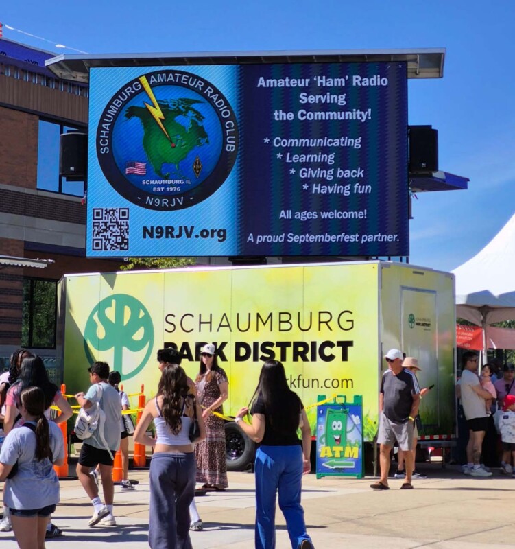
Above the Septemberfest crowd, a large screen carried a message worth celebrating: “Amateur ‘Ham’ Radio Serving the Community!” Beside the Schaumburg Amateur Radio Club’s logo were four simple commitments: communicating, learning, giving back, and having fun.
The photograph from Schaumburg’s 2026 Septemberfest captures that message above a Schaumburg Park District trailer, with festivalgoers passing below. At the bottom of the display, a short line brings the story home: “A proud Septemberfest partner.”
For the Schaumburg Amateur Radio Club, known as SARC, that partnership had a practical purpose. The club organized volunteers for public-service communication support during the September 5–7 celebration. Behind the public recognition was the work of preparing assignments, equipping volunteers, and answering the Village’s request for help.[1]
Members Stepped Forward Before the Festival Began
One of the clearest examples of SARC’s commitment appears in the club’s August 20 business meeting minutes.
Howard Mitchell, KD9WSV, brought the materials volunteers would need for Septemberfest: numbered identification cards, parking passes, food discount tickets, and loaner vests. Members were asked to collect their assigned items, with badges and vests to be returned after the event.
Then came a small moment that says a great deal about the club. Howard reported that just one volunteer slot remained open for the three-day event. Eliot Libner, N9EPA, volunteered to cover it.[2]
A schedule becomes a commitment when someone puts a name beside an assignment. That final offer of help is a concrete example of members taking responsibility for the work their club had agreed to support.
At the September 2 board meeting, Howard’s planning update confirmed that the Village of Schaumburg had again requested SARC’s support for all three days. The minutes also thanked members who had volunteered.[3]
What Amateur Radio Contributes to a Community Event
For someone new to ham radio, its role at a festival may not be obvious. SARC’s public-service work helps people at different locations exchange information through an organized radio network. The value comes from operators who listen carefully, report clearly, and know how to work together.[4]
The club’s 2026 Septemberfest guidance described possible assignments such as providing location updates, passing along observations, relaying requests, and maintaining contact with Net Control—the station coordinating radio traffic. Exact responsibilities depended on each assignment and the event coordinator’s instructions.[1]
That guidance defined a supporting role: volunteers were to observe, communicate accurately, and follow the event’s command structure. Police, fire, medical, and Village personnel retained their own responsibilities.
It is useful, disciplined work. A clear report can give an organizer information from a location they cannot see. An acknowledged instruction helps everyone know what happens next. Those ordinary exchanges explain why practiced communication belongs in the planning of a busy public event.
A Celebration With Many Moving Parts
Local coverage helps put that preparation in perspective. The Daily Herald identified 2026 as Schaumburg’s 55th annual Septemberfest, with a program spanning September 5–7 at the Al Larson Cultural Center and Robert O. Atcher Municipal Campus.
Its preview listed concerts, Taste of Schaumburg, arts and crafts, a Sunday drone show, and Monday’s Labor Day parade. The main-stage lineup included Night Ranger, White Lion, Warrant, and Max Weinberg’s Jukebox.[5]
A separate Village notice published by the Daily Herald detailed temporary road closures and parking restrictions, including additional changes for the September 7 parade along Summit Drive.[6]
Together, those reports illustrate the coordination behind the celebration. Entertainment schedules, vehicle access, parade movements, and volunteer reporting locations all require preparation. In that setting, SARC’s commitment to organized communication had a clear purpose.
A Partnership Built Through Previous Service
SARC brought an established Septemberfest relationship into 2026. The club’s earlier records document both the time members gave and the preparation behind their assignments.
Documented SARC Septemberfest service in earlier years
Year
Reported contribution
2024
13 volunteers and more than 93 hours, including preparation and event operations, supporting the Septemberfest parade.[7]
2025
26 volunteers and more than 80 service hours, according to a Village recognition notice reproduced in SARC’s December board minutes.[8]
The 2024 report describes advance radio testing, communication between assigned locations and event command, and suggestions gathered afterward to improve future participation. In 2025, Village Emergency Management and Accreditation Manager Tracy Raimondo presented the club with a plaque recognizing its service.[7][8]
These are earlier-year records, rather than totals for 2026. They show the experience and continuing relationship behind this year’s volunteer effort.
Fifty Years of Radio, Friendship, and Giving Back
The Septemberfest partnership also fits a larger SARC milestone: the club’s 50th anniversary in 2026. Its anniversary article celebrates five decades of learning, operating, friendship, and public service.[9]
The festival photograph makes that tradition visible to people who may never have attended a club meeting. It presents amateur radio as something approachable and useful, with an invitation that needs little explanation: “All ages welcome!”
That is an encouraging introduction to the hobby. Someone passing the display might be interested in electronics, curious about communicating over the air, or looking for a meaningful way to volunteer. SARC offers a place to begin that conversation.
Thank You to the People Behind the Partnership
Thank you to the SARC members who made time for Septemberfest, to Howard Mitchell for coordinating the documented preparations, and to Eliot Libner for stepping forward when the final assignment needed a volunteer. Thanks also go to the Village staff, event organizers, public-safety personnel, and fellow volunteers whose work supports Schaumburg’s community celebrations.
The message on the screen deserves to carry beyond Labor Day weekend. Communicating, learning, giving back, and having fun are all reasons to get involved.
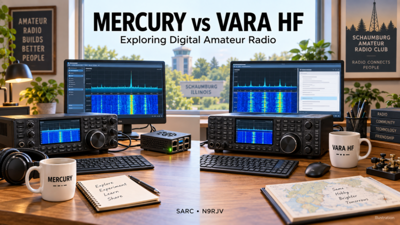
Here is a useful operating idea for Schaumburg Amateur Radio Club members: explore two ways to send messages and files over HF radio. Mercury and VARA HF offer an opportunity to learn about digital communications, compare station setups, and help newer hams make their first data connection.
The practical starting point is your intended contact. If that station uses VARA HF, choose VARA HF. If you and a partner want to explore an open-source modem, Mercury is worth a coordinated trial. The distinction between software compatibility and radio compatibility explains why.
Topic Snapshot
Mercury vs. VARA at a glance
Subject
Mercury VS VARA
Post idea from
Paul Meyes — KE9EJX
Audience
SARC members, visitors, new hams, the public, operators, and volunteers
Focus
HF messaging, file transfer, Winlink considerations, and peer-to-peer experiments
Suggested activity
A paired station demonstration followed by repeatable comparison tests
Review date
September 18, 2026. Check official documentation before installing or purchasing software.
Scope
This comparison concerns VARA HF. VARA FM and VARA SAT are separate products.[1]
What Do These Modems Do?
A software modem converts computer data into audio that a radio can transmit. At the other station, another modem decodes the received audio. HF means high frequency; these programs use a suitable single-sideband, or SSB, radio and an audio connection.
Both Mercury and VARA HF use orthogonal frequency division multiplexing, or OFDM. In simple terms, information travels on multiple closely spaced carriers. Sharing that general technique does not make their radio signals interchangeable.[2][1]
Mercury also documents automatic repeat request, or ARQ: the receiving station acknowledges data, and unsuccessful transfers can trigger another attempt. Its connected link takes turns transmitting and adjusts payload modes as conditions change.[3]
Mercury and VARA HF: The Main Tradeoffs
Features that affect a club station’s choice
Consideration
Mercury
VARA HF
License and cost
Free, open-source software with a GPL-3.0 project license.[4]
Proprietary software with a restricted free mode and a paid license for higher speeds. Check current terms with the developer.[1]
Operating systems
The project documents Linux, Windows, macOS, and Raspberry Pi support. Installation depends on the operating system and processor.[5]
A Windows modem. Linux operation can use Wine, a Windows compatibility layer; Pat documents that approach.[6]
Application connection
Provides a VARA-style command and data interface, with some commands accepted without implementing the corresponding feature.[7]
Explicitly supported by Winlink Express and used by VarAC.[8][9]
Software development
Members can inspect the code and contribute under its license.[4]
Changes to the modem depend on its developer; it is not an open-source project.[1]
Suggested club use
Coordinated experiments, native platform trials, and learning how a modem works.
Contacts and exercises whose destination already requires VARA HF.
Mercury: What Works in Its Favor?
Mercury is developed by Rhizomatica as part of its HERMES project. Native support across several operating systems gives members flexibility when choosing a computer for their station.[5]
Its open-source license also creates a useful learning opportunity. A technically curious member can inspect an implementation, suggest improvements, or contribute a fix. For a club workshop, that makes software development part of the radio experiment.[4]
Meanwhile, Mercury’s release history shows work on audio handling, radio keying, client connections, and its graphical interface. Recent releases include chat-related improvements. Check the documentation for the exact release you install.[10]
Where Mercury Needs Careful Planning
Mercury needs a compatible Mercury station at the far end. Changing your local modem does not convert a VARA-only gateway into a Mercury gateway. That follows from Mercury’s own radio protocol and its separate VARA-style application interface.[3]
In addition, active development means instructions and behavior can change between releases. Recent fixes involving Pat connections and audio devices are good reasons to record both stations’ versions and repeat a short test after updating.[10]
VARA HF: What Works in Its Favor?
VARA HF has a clearly documented role in existing applications. Winlink Express lists it as a supported radio mode. VarAC provides a separate application for conversations and other messaging features over VARA.[8][9]
Consequently, VARA is a practical starting choice when your intended gateway or operating partner already uses it. You can focus the first session on setting up audio, making a connection, and completing a message exchange.
Where VARA HF Has Tradeoffs
Its proprietary license limits opportunities to inspect or modify the modem. Higher-speed operation also involves paid registration. Confirm current licensing details on the developer’s website before buying.[1]
Linux users should plan for an additional compatibility layer. Pat can run natively on Linux, but that does not make the VARA modem itself a native Linux application. Raspberry Pi installations require particular attention to the instructions for their processor and operating system.[6][1]
Compatibility: Check All Three Layers
Mercury provides a TCP TNC interface: a network connection through which an application controls a terminal node controller, implemented here in software. Its documented defaults are port 8300 for commands and 8301 for data. TCP stands for Transmission Control Protocol.[7]
However, matching commands is only one part of a working connection. For example, Mercury’s command reference says its compression command is acknowledged without enabling modem compression. Treat compatibility as something to verify with your chosen application and release.[7]
Three separate compatibility questions
Layer
Question to answer
Application to modem
Can the client control this modem and exchange data through the configured ports?
Radio link
Are both stations using compatible modem protocols, releases, and bandwidth settings?
Message service
Do both ends support the intended email, chat, or file-transfer application?
What About Winlink Express, Pat, and VarAC?
Winlink Express and Pat both document VARA support. Mercury’s interface makes integration possible, but a successful local client connection does not establish access to a remote Winlink gateway. Confirm Mercury support at the destination before attempting a Mercury session.[8][6][7]
Similarly, VarAC and VARA are different programs. VarAC supplies the user-facing chat experience; VARA supplies the modem. VarAC’s published prerequisites identify VARA HF or VARA FM. Mercury release notes mention VarAC beacon support, but that alone does not establish complete compatibility with every VarAC feature.[9][11][10]
Which One Should You Try First?
Start with the destination and work backward. This decision guide applies the compatibility checks above.
flowchart TD
    A["Choose a contact or gateway"] --> B{"Destination requires VARA HF?"}
    B -->|Yes| C["Use VARA HF"]
    B -->|No| D{"Mercury partner confirmed?"}
    D -->|Yes| E["Match Mercury releases and settings"]
    D -->|No| F["Arrange a compatible partner"]
    F --> A
    C --> G["Check client, audio, and radio keying"]
    E --> G
    G --> H["Exchange a short test message"]
Choose a modem that matches the destination, then verify the complete station setup.
Performance: Measure the Completed Message
Claims that Mercury always matches or beats VARA HF go beyond what the documentation reviewed here establishes. Mercury publishes mode-level measurements under specified simulated conditions. Those measurements are useful, but they do not establish a universal winner against VARA on real radio paths.[2]
For a useful comparison, distinguish the displayed modem rate from goodput: the useful information delivered per unit of time. Connection setup, acknowledgments, retries, and changing conditions affect the completed transfer. Mercury’s documentation explicitly distinguishes payload rates from ARQ goodput.[2]
Also record signal-to-noise ratio, or SNR, which compares signal strength with background noise. Treat readings from different programs cautiously unless their measurement methods and reference bandwidths match.
A Suggested SARC Comparison Test
Keep the station arrangement consistent. Use the same two stations, antennas, band, and comparable occupied bandwidth. Record transmitter settings and actual power measurements where available.
Record the software. Include the application, modem release, operating system, and whether VARA is registered or operating with free-mode restrictions.
Send identical content. Begin with a short text message, then try a modest file. Record any compression settings.
Alternate the order. Run Mercury, then VARA, and reverse that order on the next pair of trials. Repeat in both directions to reduce the influence of changing conditions.
Count failures too. Record unsuccessful connections, incomplete transfers, and manual intervention. Check that the received content matches the original.
Suggested measurements for each trial
Measurement
Why record it?
Connection success
Shows how often a usable session begins.
Time to complete
Measures from the connection attempt to confirmed delivery.
Correct delivery
Checks the text or compares a file checksum, a compact fingerprint of its contents.
Operator effort
Records configuration problems, restarts, and recovery steps.
Present the results as observations from those stations and conditions. A small club trial can guide local choices without proving that one modem is best everywhere.
How to Participate
Begin by telling a potential test partner which computer you plan to use and whether your goal is email, chat, or file transfer. Then agree on the modem, application, and software versions.
For a station demonstration, prepare a suitable HF radio, antenna, computer, radio audio connection, and the required cables. Follow the radio and modem instructions for audio levels and push-to-talk, or PTT, which switches the transmitter on. Mercury documents several PTT methods; the appropriate choice depends on your interface.[5]
Ask an experienced operator to help select an appropriate frequency and station settings. Listen before transmitting, begin with a short exchange, and keep notes. Visitors can follow the decoded messages or record results while the station operator handles the radio.
Suggested SARC Goals
Ways different participants can contribute
Participant
Suggested goal
Useful result
New hams
Trace a message from the application through the modem to the receiving station.
Explain the difference between the application and the radio protocol.
Visitors and the public
Observe a message exchange and ask how the stations connect.
See a practical example of digital amateur radio.
Linux and Raspberry Pi users
Try Mercury on a supported setup with a confirmed partner.
Write a repeatable installation and configuration checklist.
Winlink and chat operators
Confirm the destination’s requirements before changing modems.
Complete the intended message workflow.
Emergency communications volunteers
Practice a short exercise message using the group’s agreed software.
Document delivery, recovery, and operator handoff.
Technical members and helpers
Run paired tests and help others reproduce the setup.
Share measurements and clear troubleshooting notes.
Give It a Try
Choose one achievable goal: send a short message, complete a file transfer, or help another member understand the station. Mercury offers an interesting path for experimentation, while VARA HF remains the appropriate choice for destinations using VARA.
Bring your questions and a willingness to compare notes. Share which computer you use, what you want to send, and what worked. Those practical details can help the next SARC member get on the air with confidence.
The SARC Picnic Sunday, August 30th at the reserved cabin in Bartlett.
We had plenty of room to eat, relax, catch up with friends, and enjoy the afternoon.
What a year it has been for SARC.Our members have stepped up again and again to support our community, providing communications assistance for events like the Chicagoland Marathon, the MS Society, the Hoffman Estates Fourth of July Parade, and many others.
When our community called, SARC answered — and we did a fantastic job. Se we celebrated with some good company, and celebrate the work we’ve done together.